Boston House Pricing Prediction

import matplotlib.pyplot as plt
from sklearn_genetic import GASearchCV
from sklearn_genetic.space import Integer, Categorical, Continuous
from sklearn_genetic.plots import plot_fitness_evolution, plot_search_space
from sklearn_genetic.callbacks import LogbookSaver, ProgressBar
from sklearn.datasets import load_boston
from sklearn.model_selection import train_test_split, KFold
from sklearn.tree import DecisionTreeRegressor
from sklearn.metrics import r2_score
from sklearn.pipeline import Pipeline
from sklearn.preprocessing import StandardScaler

Import the data and split it in train and test sets

data = load_boston()

y = data["target"]
X = data["data"]

X_train, X_test, y_train, y_test = train_test_split(X, y, test_size=0.33, random_state=42)

Define the classifier to tune

clf = DecisionTreeRegressor()
pipe = Pipeline([("scaler", StandardScaler()), ("clf", clf)])

Create the CV strategy and define the param grid

cv = KFold(n_splits=5, shuffle=True)

param_grid = {
    "clf__ccp_alpha": Continuous(0, 1),
    "clf__criterion": Categorical(["mse", "mae"]),
    "clf__max_depth": Integer(2, 20),
    "clf__min_samples_split": Integer(2, 30)}

Define the GASearchCV options

evolved_estimator = GASearchCV(
    estimator=pipe,
    cv=3,
    scoring="r2",
    population_size=15,
    generations=20,
    tournament_size=3,
    elitism=True,
    keep_top_k=4,
    crossover_probability=0.9,
    mutation_probability=0.05,
    param_grid=param_grid,
    criteria="max",
    algorithm="eaMuCommaLambda",
    n_jobs=-1)

Optionally, create some Callbacks

callbacks = [LogbookSaver(checkpoint_path="./logbook.pkl"), ProgressBar()]

Fit the model and see some results

evolved_estimator.fit(X_train, y_train, callbacks=callbacks)
y_predict_ga = evolved_estimator.predict(X_test)
r_squared = r2_score(y_test, y_predict_ga)

gen     nevals  fitness         fitness_std     fitness_max     fitness_min
0       15      0.616334        0.0737326       0.699908        0.520033
1       29      0.677235        0.0439198       0.708851        0.520033
2       30      0.694427        0.0193834       0.738255        0.6749
3       29      0.699751        0.0154815       0.727109        0.676053
4       28      0.701338        0.00901281      0.713701        0.680425
5       28      0.698859        0.00957983      0.714697        0.683542
6       29      0.696912        0.0104028       0.709564        0.680759
7       26      0.705685        0.00819244      0.714573        0.683011
8       29      0.70907         0.00473398      0.714573        0.699808
9       28      0.708067        0.00616905      0.714526        0.695999
10      27      0.70679         0.00423967      0.711368        0.694636
11      30      0.702428        0.0053359       0.710461        0.695597
12      27      0.709388        0.00359735      0.713665        0.703131
13      29      0.701775        0.00600001      0.707575        0.691636
14      30      0.703581        0.00699099      0.712533        0.692699
15      29      0.705634        0.00417138      0.709928        0.692095
16      29      0.706242        0.00383751      0.709808        0.694379
17      29      0.7077          0.00347843      0.711972        0.699101
18      28      0.706694        0.00608173      0.712897        0.690798
19      28      0.706568        0.00477195      0.712003        0.69356
20      30      0.706721        0.00587165      0.71358         0.694205

print(evolved_estimator.best_params_)
print("r-squared: ", "{:.2f}".format(r_squared))
print("Best k solutions: ", evolved_estimator.hof)

{'clf__ccp_alpha': 0.014034324281064214, 'clf__criterion': 'mae', 'clf__max_depth': 18, 'clf__min_samples_split': 12}
r-squared:  0.67
Best k solutions:  {0: {'clf__ccp_alpha': 0.014034324281064214, 'clf__criterion': 'mae', 'clf__max_depth': 18, 'clf__min_samples_split': 12}, 1: {'clf__ccp_alpha': 0.12139328299577712, 'clf__criterion': 'mae', 'clf__max_depth': 15, 'clf__min_samples_split': 3}, 2: {'clf__ccp_alpha': 0.014034324281064214, 'clf__criterion': 'mae', 'clf__max_depth': 9, 'clf__min_samples_split': 3}, 3: {'clf__ccp_alpha': 0.014034324281064214, 'clf__criterion': 'mae', 'clf__max_depth': 14, 'clf__min_samples_split': 3}}

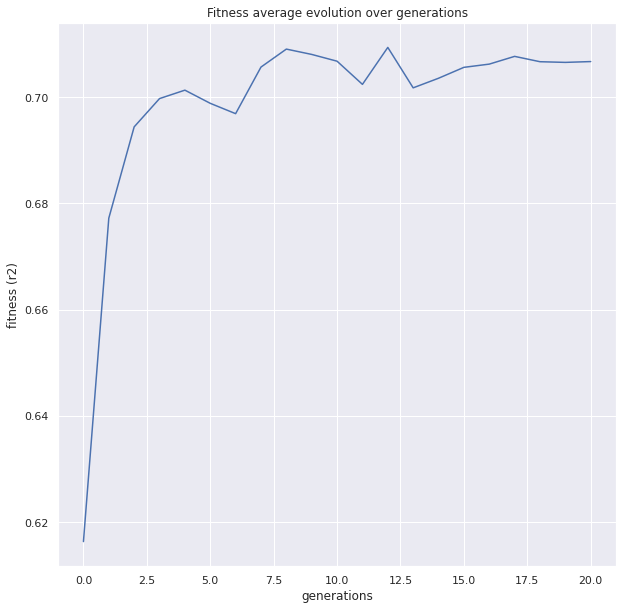
plot = plot_fitness_evolution(evolved_estimator, metric="fitness")
plt.show()

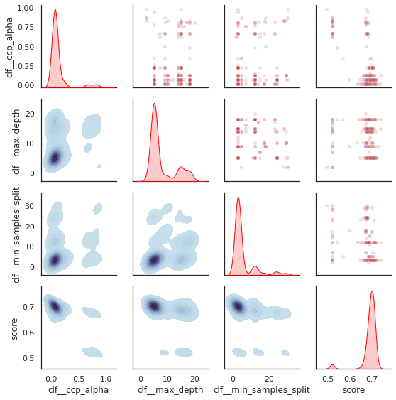
plot_search_space(evolved_estimator)
plt.show()