Pipeline Prediction
[ ]:
import matplotlib.pyplot as plt
from sklearn_genetic import GASearchCV
from sklearn_genetic.space import Integer, Categorical, Continuous
from sklearn_genetic.plots import plot_fitness_evolution, plot_search_space
from sklearn_genetic.callbacks import LogbookSaver, ProgressBar
from sklearn.datasets import load_diabetes
from sklearn.model_selection import train_test_split, KFold
from sklearn.ensemble import GradientBoostingRegressor
from sklearn.metrics import mean_squared_error
from sklearn.pipeline import Pipeline
from sklearn.preprocessing import StandardScaler
Import the data and split it in train and test sets
[2]:
data = load_diabetes()

y = data["target"]
X = data["data"]

X_train, X_test, y_train, y_test = train_test_split(X, y, test_size=0.33, random_state=42)
Define the regressor to tune
[3]:
rg = GradientBoostingRegressor()
pipe = Pipeline([("scaler", StandardScaler()), ("rg", rg)])
Create the CV strategy and define the param grid
[4]:
cv = KFold(n_splits=5, shuffle=True)

param_grid = {
    "rg__n_estimators": Integer(50, 600),
    "rg__loss": Categorical(["absolute_error", "squared_error"]),
    "rg__max_depth": Integer(2, 10),
    "rg__learning_rate": Continuous(0.001, 0.01, distribution="log-uniform")}
Define the GASearchCV options
[5]:
evolved_estimator = GASearchCV(
    estimator=pipe,
    cv=cv,
    scoring="neg_mean_squared_error",
    population_size=8,
    generations=15,
    tournament_size=3,
    elitism=True,
    keep_top_k=4,
    crossover_probability=0.9,
    mutation_probability=0.08,
    param_grid=param_grid,
    criteria="max",
    algorithm="eaMuCommaLambda",
    n_jobs=-1)
Optionally, create some Callbacks
[6]:
callbacks = [LogbookSaver(checkpoint_path="./logbook.pkl")]
Fit the model and see some results
[7]:
evolved_estimator.fit(X_train, y_train, callbacks=callbacks)
y_predict_ga = evolved_estimator.predict(X_test)
mse = mean_squared_error(y_test, y_predict_ga)
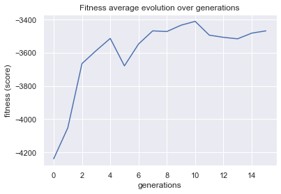
gen     nevals  fitness         fitness_std     fitness_max     fitness_min
0       8       -4238.26        565.058         -3756.78        -5523.09
1       16      -4051.7         352.254         -3756.29        -4631.79
2       16      -3665.2         70.1723         -3572.13        -3749.68
3       16      -3587.2         49.7041         -3507.56        -3644.64
4       16      -3513.45        102.322         -3420.14        -3698.88
5       16      -3678.71        164.066         -3521.83        -4011.67
6       15      -3547.3         35.2384         -3500.55        -3604.69
7       16      -3468.1         51.9507         -3379.15        -3542.45
8       16      -3472.2         51.3204         -3410.31        -3581.8
9       16      -3434.18        43.9115         -3371.14        -3514.54
10      16      -3410.84        94.4055         -3325.11        -3560.57
11      16      -3493.9         93.8796         -3393.02        -3662.27
12      16      -3506.98        32.4934         -3478.73        -3588.94
13      16      -3515.91        133.628         -3300.73        -3696.27
14      16      -3481.82        58.9704         -3399.49        -3616.37
15      16      -3468.11        10.7602         -3450.02        -3476.26
[8]:
print(evolved_estimator.best_params_)
print("mse: ", "{:.2f}".format(mse))
print("Best k solutions: ", evolved_estimator.hof)
{'rg__n_estimators': 561, 'rg__loss': 'squared_error', 'rg__max_depth': 3, 'rg__learning_rate': 0.006219524925263899}
mse:  3169.70
Best k solutions:  {0: {'rg__n_estimators': 561, 'rg__loss': 'squared_error', 'rg__max_depth': 3, 'rg__learning_rate': 0.006219524925263899}, 1: {'rg__n_estimators': 504, 'rg__loss': 'squared_error', 'rg__max_depth': 3, 'rg__learning_rate': 0.006219524925263899}, 2: {'rg__n_estimators': 517, 'rg__loss': 'squared_error', 'rg__max_depth': 3, 'rg__learning_rate': 0.006219524925263899}, 3: {'rg__n_estimators': 561, 'rg__loss': 'squared_error', 'rg__max_depth': 3, 'rg__learning_rate': 0.004507098298712037}}
[9]:
plot = plot_fitness_evolution(evolved_estimator, metric="fitness")
plt.show()
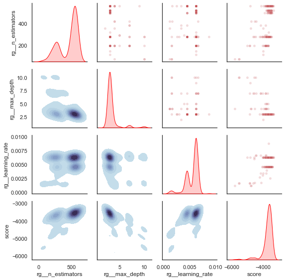
[10]:
plot_search_space(evolved_estimator)
plt.show()
[ ]: