Using Adapters
Introduction
You can define adapters to have a dynamic mutation and crossover probabilities over the optimization instead of a fixed value. The idea is to make these probabilities a function of the generations; this definition can enable different training strategies, for example:
Start with a high probability mutation to explore more diverse solutions and slowly reduce it to stay with the more promising ones.
Start with a low crossover and end with a higher probability
Combine different strategies for each parameter
All the methods uses three parameters:
initial_value: This is the value used at generation 0
end_value: It’s the limit value that the parameter can take, starting from initial_value
adaptive_rate: Controls how fast the value approaches the end_value; greater values increase the speed of convergence
For the following sections, it’s important to understand this notation:
Name |
Notation |
|---|---|
initial_value |
\(p_0\) |
end_value |
\(p_f\) |
current generation |
\(t\) |
adaptive_rate |
\(\alpha\) |
value at generation t |
\(p(t; \alpha)\) |
Note that \(p_0\) doesn’t need to be greater than \(p_f\).
If \(p_0 > p_f\), you are performing a decay towards \(p_f\).
If \(p_0 < p_f\), you are performing an ascend towards \(p_f\).
All the non-constant adapters \(p(t; \alpha)\), for \(\alpha \in (0,1)\), have the following properties:
The following adapters are available:
ConstantAdapter
ExponentialAdapter
InverseAdapter
PotentialAdapter
ConstantAdapter
This adapter is meant to be used internally by the package; when the user doesn’t create an adapter but instead defines the crossover or mutation probability as a real number, the package will convert it to a ConstantAdapter, so the library can use the internal API with the same methods in both cases. Because of this, its definition is:
ExponentialAdapter
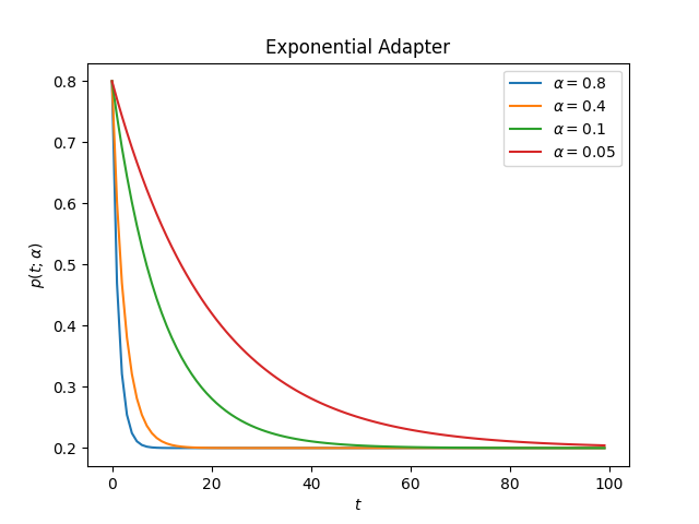
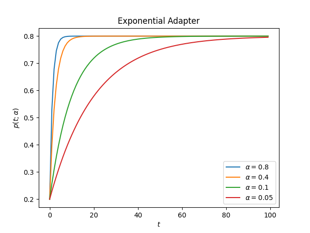
The Exponential Adapter uses the following form to change the initial value
Usage example:
from sklearn_genetic.schedules import ExponentialAdapter

# Decay over initial_value
adapter = ExponentialAdapter(initial_value=0.8, end_value=0.2, adaptive_rate=0.1)

# Run a few iterations
for _ in range(3):
    adapter.step()  # 0.8, 0.74, 0.69
This is how the adapter looks for different values of alpha
decay:
ascend:
import matplotlib.pyplot as plt
from sklearn_genetic.schedules import ExponentialAdapter

values = [{"initial_value": 0.8, "end_value": 0.2},  # Decay
          {"initial_value": 0.2, "end_value": 0.8}]  # Ascend
alphas = [0.8, 0.4, 0.1, 0.05]

for value in values:
    for alpha in alphas:
        adapter = ExponentialAdapter(**value, adaptive_rate=alpha)
        adapter_result = [adapter.step() for _ in range(100)]

        plt.plot(adapter_result, label=r'$\alpha={}$'.format(alpha))

    plt.xlabel(r'$t$')
    plt.ylabel(r'$p(t; \alpha)$')
    plt.title("Exponential Adapter")
    plt.legend()
    plt.show()
InverseAdapter
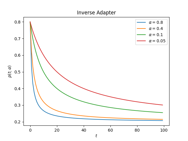
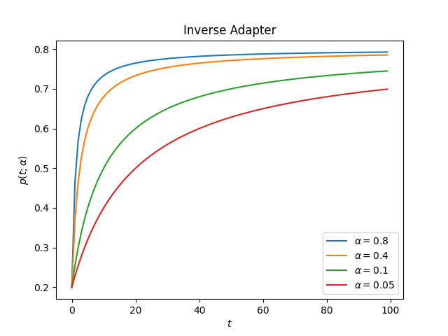
The Inverse Adapter uses the following form to change the initial value
Usage example:
from sklearn_genetic.schedules import InverseAdapter

# Decay over initial_value
adapter = InverseAdapter(initial_value=0.8, end_value=0.2, adaptive_rate=0.1)

# Run a few iterations
for _ in range(3):
    adapter.step()  # 0.8, 0.75, 0.7
This is how the adapter looks for different values of alpha
decay:
ascend:
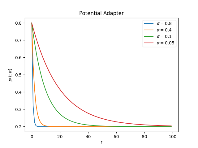
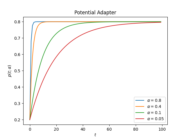
PotentialAdapter
The Inverse Adapter uses the following form to change the initial value
Usage example:
from sklearn_genetic.schedules import PotentialAdapter

# Decay over initial_value
adapter = PotentialAdapter(initial_value=0.8, end_value=0.2, adaptive_rate=0.1)

# Run a few iterations
for _ in range(3):
    adapter.step()  # 0.8, 0.26, 0.206
This is how the adapter looks for different values of alpha
decay:
ascend:
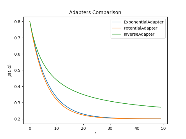
Compare
This is how all adapters looks like for the same value of alpha
decay:
ascend:
import matplotlib.pyplot as plt
from sklearn_genetic.schedules import ExponentialAdapter, PotentialAdapter, InverseAdapter


params = {"initial_value": 0.2, "end_value": 0.8, "adaptive_rate": 0.15}  # Ascend
adapters = [ExponentialAdapter(**params), PotentialAdapter(**params), InverseAdapter(**params)]

for adapter in adapters:
    adapter_result = [adapter.step() for _ in range(50)]

    plt.plot(adapter_result, label=f"{type(adapter).__name__}")

plt.xlabel(r'$t$')
plt.ylabel(r'$p(t; \alpha)$')
plt.title("Adapters Comparison")
plt.legend()
plt.show()
Full Example
In this example, we want to create a decay strategy for the mutation probability, and an ascend strategy for the crossover probability, lets call them \(p_{mt}(t; \alpha)\) and \(p_{cr}(t; \alpha)\) respectively; this will enable the optimizer to explore more diverse solutions in the first iterations. Take into account that on this scenario, we must be careful on choosing \(\alpha, p_0, p_f\), this is because the evolutionary implementation requires that:
The same idea can be used for hypeparameter tuning or feature selection.
from sklearn_genetic import GASearchCV
from sklearn_genetic import ExponentialAdapter
from sklearn_genetic.space import Continuous, Categorical, Integer
from sklearn.ensemble import RandomForestClassifier
from sklearn.model_selection import train_test_split, StratifiedKFold
from sklearn.datasets import load_digits
from sklearn.metrics import accuracy_score

data = load_digits()
n_samples = len(data.images)
X = data.images.reshape((n_samples, -1))
y = data['target']
X_train, X_test, y_train, y_test = train_test_split(X, y, test_size=0.33, random_state=42)

clf = RandomForestClassifier()

mutation_adapter = ExponentialAdapter(initial_value=0.8, end_value=0.2, adaptive_rate=0.1)
crossover_adapter = ExponentialAdapter(initial_value=0.2, end_value=0.8, adaptive_rate=0.1)

param_grid = {'min_weight_fraction_leaf': Continuous(0.01, 0.5, distribution='log-uniform'),
              'bootstrap': Categorical([True, False]),
              'max_depth': Integer(2, 30),
              'max_leaf_nodes': Integer(2, 35),
              'n_estimators': Integer(100, 300)}

cv = StratifiedKFold(n_splits=3, shuffle=True)

evolved_estimator = GASearchCV(estimator=clf,
                               cv=cv,
                               scoring='accuracy',
                               population_size=20,
                               generations=25,
                               mutation_probability=mutation_adapter,
                               crossover_probability=crossover_adapter,
                               param_grid=param_grid,
                               n_jobs=-1)

# Train and optimize the estimator
evolved_estimator.fit(X_train, y_train)
# Best parameters found
print(evolved_estimator.best_params_)
# Use the model fitted with the best parameters
y_predict_ga = evolved_estimator.predict(X_test)
print(accuracy_score(y_test, y_predict_ga))

# Saved metadata for further analysis
print("Stats achieved in each generation: ", evolved_estimator.history)
print("Best k solutions: ", evolved_estimator.hof)