Using Adapters

Introduction

Adapters let you change the mutation and crossover probabilities as the optimization progresses, instead of keeping them fixed for every generation. In practice, an adapter is a small schedule that returns a new probability at each generation.

This makes it possible to express different search strategies, for example:

Start with a high mutation probability to explore more diverse solutions, then slowly reduce it to refine the most promising candidates.
Start with a low crossover probability and increase it over time.
Use different schedules for mutation and crossover.

All adapters use three parameters:

initial_value: value used at generation 0.
end_value: target value approached by the schedule.
adaptive_rate: controls how quickly the schedule approaches end_value. Larger values make the schedule change faster.

The following notation is used throughout this tutorial:

Name	Notation
initial_value	\(p_0\)
end_value	\(p_f\)
current generation	\(t\)
adaptive_rate	\(\alpha\)
value at generation t	\(p(t; \alpha)\)

The initial value \(p_0\) does not need to be greater than the final value \(p_f\).

If \(p_0 > p_f\), the adapter defines a decay toward \(p_f\).

If \(p_0 < p_f\), the adapter defines an ascent toward \(p_f\).

All non-constant adapters \(p(t; \alpha)\), for \(\alpha \in (0,1)\), have the following properties:

\[\begin{split}\lim_{t \to 0^{+}} p(t; \alpha) = p_0\\ \\ \lim_{t \to +\infty} p(t; \alpha) = p_f\end{split}\]

The following adapters are available:

ConstantAdapter
ExponentialAdapter
InverseAdapter
PotentialAdapter

ConstantAdapter

This adapter is mainly used internally by the package. When you pass the crossover or mutation probability as a real number, the package converts that number into a ConstantAdapter. This lets the optimization code use the same internal API for both fixed probabilities and scheduled probabilities.

Its definition is:

\[p(t; \alpha) = p_0\]

ExponentialAdapter

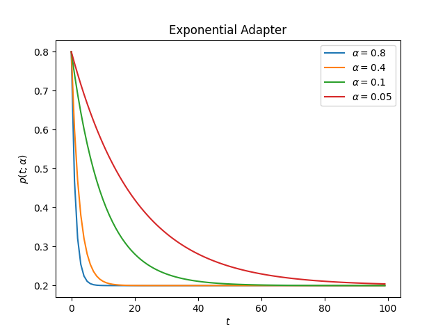
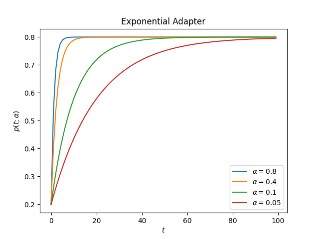
The ExponentialAdapter changes the probability exponentially:

\[p(t; \alpha) = (p_0-p_f)e^{-\alpha t} + p_f\]

Usage example:

from sklearn_genetic.schedules import ExponentialAdapter

# Decay from initial_value toward end_value
adapter = ExponentialAdapter(initial_value=0.8, end_value=0.2, adaptive_rate=0.1)

# Run a few iterations
for _ in range(3):
    adapter.step()  # 0.8, 0.74, 0.69

The following plots show the adapter for different values of \(\alpha\). Larger values of \(\alpha\) move toward the target value more quickly.

decay:

ascent:

import matplotlib.pyplot as plt
from sklearn_genetic.schedules import ExponentialAdapter

values = [{"initial_value": 0.8, "end_value": 0.2},  # Decay
          {"initial_value": 0.2, "end_value": 0.8}]  # Ascent
alphas = [0.8, 0.4, 0.1, 0.05]

for value in values:
    for alpha in alphas:
        adapter = ExponentialAdapter(**value, adaptive_rate=alpha)
        adapter_result = [adapter.step() for _ in range(100)]

        plt.plot(adapter_result, label=r'$\alpha={}$'.format(alpha))

    plt.xlabel(r'$t$')
    plt.ylabel(r'$p(t; \alpha)$')
    plt.title("Exponential Adapter")
    plt.legend()
    plt.show()

InverseAdapter

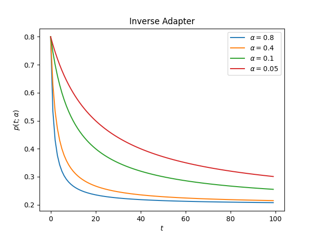
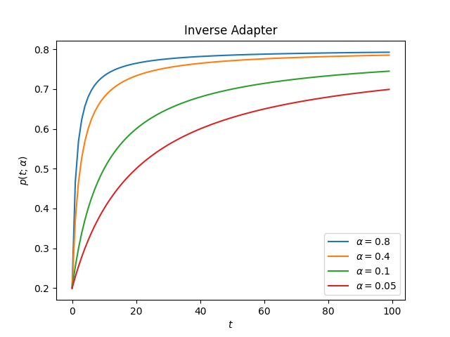
The InverseAdapter changes the probability with inverse decay:

\[p(t; \alpha) = \frac{(p_0-p_f)}{1+\alpha t} + p_f\]

Usage example:

from sklearn_genetic.schedules import InverseAdapter

# Decay from initial_value toward end_value
adapter = InverseAdapter(initial_value=0.8, end_value=0.2, adaptive_rate=0.1)

# Run a few iterations
for _ in range(3):
    adapter.step()  # 0.8, 0.75, 0.7

The following plots show the adapter for different values of \(\alpha\).

decay:

ascent:

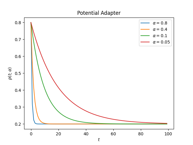
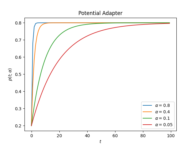
PotentialAdapter

The PotentialAdapter changes the probability with the following form:

\[p(t; \alpha) = (p_0-p_f)(1-\alpha)^{ t} + p_f\]

Usage example:

from sklearn_genetic.schedules import PotentialAdapter

# Decay from initial_value toward end_value
adapter = PotentialAdapter(initial_value=0.8, end_value=0.2, adaptive_rate=0.1)

# Run a few iterations
for _ in range(3):
    adapter.step()  # 0.8, 0.26, 0.206

The following plots show the adapter for different values of \(\alpha\).

decay:

ascent:

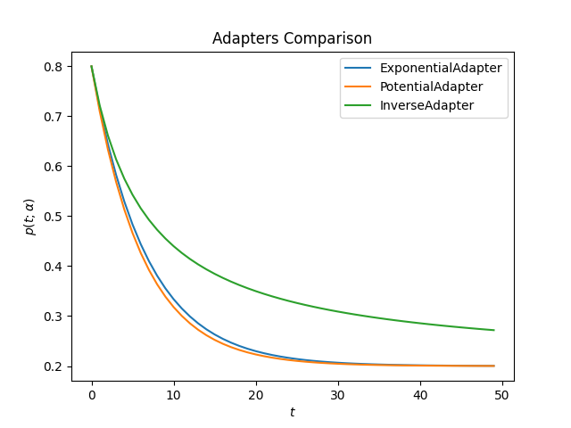
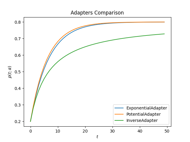
Compare

The following plots compare all adapters using the same value of \(\alpha\).

decay:

ascent:

import matplotlib.pyplot as plt
from sklearn_genetic.schedules import ExponentialAdapter, PotentialAdapter, InverseAdapter


params = {"initial_value": 0.2, "end_value": 0.8, "adaptive_rate": 0.15}  # Ascent
adapters = [ExponentialAdapter(**params), PotentialAdapter(**params), InverseAdapter(**params)]

for adapter in adapters:
    adapter_result = [adapter.step() for _ in range(50)]

    plt.plot(adapter_result, label=f"{type(adapter).__name__}")

plt.xlabel(r'$t$')
plt.ylabel(r'$p(t; \alpha)$')
plt.title("Adapters Comparison")
plt.legend()
plt.show()

Full Example

In this example, we create a decay schedule for the mutation probability and an ascent schedule for the crossover probability. Let us call them \(p_{mt}(t; \alpha)\) and \(p_{cr}(t; \alpha)\), respectively.

The recommended default is to start with high crossover (0.8) and low mutation (0.1). Crossover is the primary search operator — it recombines good parameter combinations from high-fitness parents. Mutation provides exploratory perturbation and should be kept small so that discovered good regions are refined rather than abandoned.

A useful adaptive strategy keeps crossover high and gently increases mutation later to escape stagnation. The implementation requires:

\[p_{mt}(t; \alpha) + p_{cr}(t; \alpha) <= 1; \forall t\]

The same idea can be used for hyperparameter tuning or feature selection.

from sklearn_genetic import EvolutionConfig, GASearchCV, PopulationConfig, RuntimeConfig
from sklearn_genetic.schedules import ExponentialAdapter
from sklearn_genetic.space import Continuous, Categorical, Integer
from sklearn.ensemble import RandomForestClassifier
from sklearn.model_selection import train_test_split, StratifiedKFold
from sklearn.datasets import load_digits
from sklearn.metrics import accuracy_score

data = load_digits()
n_samples = len(data.images)
X = data.images.reshape((n_samples, -1))
y = data['target']
X_train, X_test, y_train, y_test = train_test_split(X, y, test_size=0.33, random_state=42)

clf = RandomForestClassifier()

# Start with strong recombination and gentle mutation; slightly relax crossover
# over time to allow more diverse offspring if the population stagnates.
crossover_adapter = ExponentialAdapter(initial_value=0.8, end_value=0.6, adaptive_rate=0.1)
mutation_adapter = ExponentialAdapter(initial_value=0.1, end_value=0.2, adaptive_rate=0.1)

param_grid = {'min_weight_fraction_leaf': Continuous(0.01, 0.5, distribution='log-uniform'),
              'bootstrap': Categorical([True, False]),
              'max_depth': Integer(2, 30),
              'max_leaf_nodes': Integer(2, 35),
              'n_estimators': Integer(100, 300)}

cv = StratifiedKFold(n_splits=3, shuffle=True)

evolved_estimator = GASearchCV(estimator=clf,
                               cv=cv,
                               scoring='accuracy',
                               param_grid=param_grid,
                               evolution_config=EvolutionConfig(
                                   population_size=20,
                                   generations=25,
                                   crossover_probability=crossover_adapter,
                                   mutation_probability=mutation_adapter,
                               ),
                               population_config=PopulationConfig(initializer="smart"),
                               runtime_config=RuntimeConfig(n_jobs=-1))

# Train and optimize the estimator
evolved_estimator.fit(X_train, y_train)
# Best parameters found
print(evolved_estimator.best_params_)
# Use the model fitted with the best parameters
y_predict_ga = evolved_estimator.predict(X_test)
print(accuracy_score(y_test, y_predict_ga))

# Saved metadata for further analysis
print("Stats achieved in each generation: ", evolved_estimator.history)
print("Best k solutions: ", evolved_estimator.hof)