How to Use sklearn-genetic-opt
Introduction
sklearn-genetic-opt uses evolutionary algorithms to tune scikit-learn
estimators and select informative features. It works with classification and
regression estimators, including estimators inside a scikit-learn
Pipeline.
The package follows the familiar scikit-learn search API, but the search space
is defined differently from GridSearchCV.
Instead of listing every candidate value, you define the allowed range or
choices for each hyperparameter. The optimizer samples candidates from that
space, evaluates them with cross-validation, and uses evolutionary operators to
produce new candidates over several generations.
Internally, sklearn-genetic-opt uses the DEAP package. A population is a set of candidate solutions. Each candidate is evaluated, selected, crossed over, or mutated to create the next generation. The process continues until the configured number of generations is reached or a callback stops the search.
This tutorial covers the two most common workflows:
Hyperparameter tuning with
GASearchCV.Feature selection with
GAFeatureSelectionCV.
Hyperparameter Tuning
For the first example, we will tune an
MLPClassifier on the
digits dataset.
The digits dataset is a multi-class classification problem.
import matplotlib.pyplot as plt
from sklearn.datasets import load_digits
from sklearn.metrics import accuracy_score
from sklearn.model_selection import StratifiedKFold, train_test_split
from sklearn.neural_network import MLPClassifier

from sklearn_genetic import EvolutionConfig, GASearchCV, PopulationConfig, RuntimeConfig
from sklearn_genetic.space import Categorical, Continuous, Integer
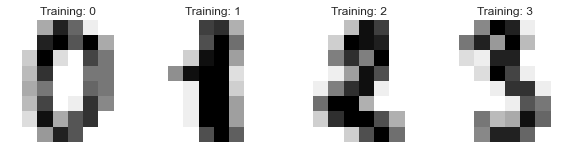
Load the data, split it into training and test sets, and visualize a few examples:
data = load_digits()
n_samples = len(data.images)
X = data.images.reshape((n_samples, -1))
y = data["target"]

X_train, X_test, y_train, y_test = train_test_split(
    X, y, test_size=0.33, random_state=42
)

_, axes = plt.subplots(nrows=1, ncols=4, figsize=(10, 3))
for ax, image, label in zip(axes, data.images, data.target):
    ax.set_axis_off()
    ax.imshow(image, cmap=plt.cm.gray_r, interpolation="nearest")
    ax.set_title("Training: %i" % label)
The samples should look like this:
Next, define the hyperparameter search space. The keys in param_grid must
match valid estimator parameters. The values are search-space dimensions:
Integersamples integer values from a range.Continuoussamples floating-point values from a range.Categoricalsamples from a fixed list of choices.
param_grid = {
    "tol": Continuous(1e-2, 1e10, distribution="log-uniform"),
    "alpha": Continuous(1e-5, 2e-5),
    "activation": Categorical(["logistic", "tanh"]),
    "batch_size": Integer(300, 350),
}
For example, batch_size can take any integer value from 300 to 350, while
activation must be either "logistic" or "tanh". The
distribution argument controls how random values are sampled from a
dimension. A log-uniform distribution is useful when a parameter spans several
orders of magnitude.
Now create the estimator and the cross-validation strategy:
clf = MLPClassifier(hidden_layer_sizes=(50, 30))

cv = StratifiedKFold(n_splits=3, shuffle=True, random_state=42)

evolved_estimator = GASearchCV(
    estimator=clf,
    cv=cv,
    scoring="accuracy",
    param_grid=param_grid,
    evolution_config=EvolutionConfig(population_size=10, generations=20),
    population_config=PopulationConfig(initializer="smart"),
    runtime_config=RuntimeConfig(n_jobs=-1, verbose=True),
)
Most arguments have the same meaning as in scikit-learn search estimators:
cv controls the validation strategy, scoring controls the metric, and
RuntimeConfig.n_jobs controls parallel execution. During the genetic search, unique
candidates in the same generation are evaluated in parallel when possible; each
candidate runs its cross-validation sequentially to avoid nested parallelism.
Set RuntimeConfig(parallel_backend="cv") to keep candidate evaluation
serial and pass n_jobs to each candidate’s cross-validation instead. The
genetic-search-specific values EvolutionConfig.population_size and EvolutionConfig.generations
determine how many candidate solutions are explored. By default,
PopulationConfig(initializer="smart") builds a more diverse initial population
using estimator defaults, warm starts when provided, Latin hypercube samples for
numeric hyperparameters, and stratified categorical values. Set
PopulationConfig(initializer="random") to use the previous random initialization
behavior. After fitting, fit_stats_ reports evaluation counters such as
cache hits, duplicate candidates, cross-validation calls, and skipped invalid
feature masks.
Run the optimization:
evolved_estimator.fit(X_train, y_train)
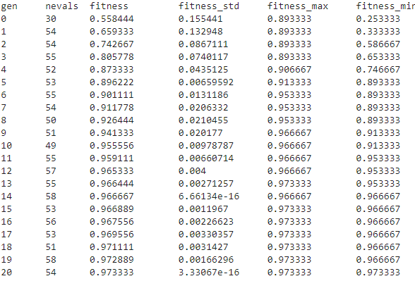
During training, you should see a generation-by-generation log:
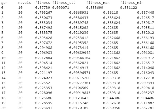
Each row summarizes one generation:
gen: generation number.
nevals: number of evaluated individuals in the generation.
fitness: average cross-validation score for the generation.
fitness_std: standard deviation of the cross-validation scores.
fitness_best: best score found so far during the full search.
fitness_max: best individual score in the generation.
fitness_min: worst individual score in the generation.
A compact summary of diversity and optimizer state appears at the right of each row:
div:
genotype_diversity— the average fraction of distinct values per gene position across the population. A value near 1.0 means the population is diverse; a value near 0.0 means it has converged to nearly identical configurations.unique:
unique_individual_ratio— the fraction of the population that are distinct individuals. Values belowdiversity_threshold(default 0.25) trigger diversity control.stag:
stagnation_generations— how many consecutive generations have passed withoutfitness_bestimproving. Useful for deciding when to add an early-stopping callback.events: a compact summary of optimizer interventions in the generation —
div(diversity control triggered),imm=N(N random immigrants injected),dup=N(N duplicates replaced),share(fitness sharing applied).
After fitting, inspect the full history as a DataFrame:
import pandas as pd

history = pd.DataFrame(evolved_estimator.history)
print(history[[
    "gen", "fitness_best", "genotype_diversity",
    "unique_individual_ratio", "stagnation_generations",
]])
And check evaluation cost via fit_stats_:
print(evolved_estimator.fit_stats_)
# evaluated_candidates: total individuals presented to the evaluator
# unique_candidates:    distinct configurations actually cross-validated
# cache_hits:           evaluations reused from the fitness cache
# random_immigrants:    individuals injected when diversity control triggered
# skipped_invalid_candidates: configs that raised exceptions during fit
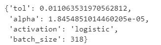
After fitting, GASearchCV behaves like a fitted scikit-learn estimator. It
uses the best hyperparameters found during the search:
print(evolved_estimator.best_params_)
y_predict_ga = evolved_estimator.predict(X_test)
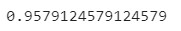
print(accuracy_score(y_test, y_predict_ga))
In this run, the test accuracy was approximately 0.96.
y_predict_ga = evolved_estimator.predict(X_test)
accuracy_score(y_test, y_predict_ga)
evolved_estimator.best_params_
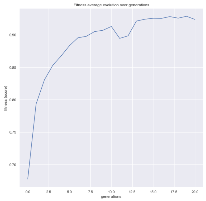
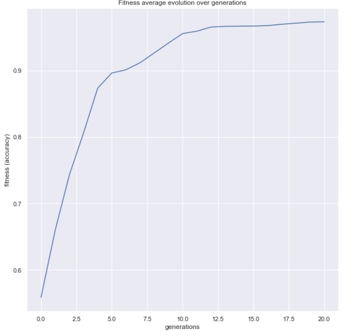
You can also inspect the optimization process. The
plot_fitness_evolution() helper shows how the
best score found so far changed over generations:
from sklearn_genetic.plots import plot_fitness_evolution

plot_fitness_evolution(evolved_estimator)
plt.show()
The evolved_estimator.logbook attribute stores the results generated during
the search. You can use plot_search_space() to see
which hyperparameter values were sampled:
from sklearn_genetic.plots import plot_search_space

plot_search_space(evolved_estimator, features=["tol", "batch_size", "alpha"])
plt.show()
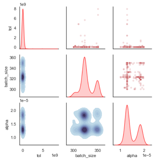
In this plot, each axis represents a sampled hyperparameter value. For example,
the tol range is intentionally broad in this tutorial, and the plot can help
you decide whether to narrow that range in a second search.
Feature Selection
For the second example, we will use the Iris dataset and add random noise features. The goal is to recover a useful subset of features while ignoring the noise.
import matplotlib.pyplot as plt
import numpy as np
from sklearn.datasets import load_iris
from sklearn.metrics import accuracy_score
from sklearn.model_selection import train_test_split
from sklearn.svm import SVC

from sklearn_genetic import (
    EvolutionConfig,
    GAFeatureSelectionCV,
    PopulationConfig,
    RuntimeConfig,
)
from sklearn_genetic.plots import plot_fitness_evolution

data = load_iris()
X, y = data["data"], data["target"]

noise = np.random.uniform(0, 10, size=(X.shape[0], 10))
X = np.hstack((X, noise))

X_train, X_test, y_train, y_test = train_test_split(
    X, y, test_size=0.33, random_state=0
)
The resulting dataset contains the original Iris features plus 10 noisy features.
GAFeatureSelectionCV is similar to GASearchCV, but it does not optimize
hyperparameters. Instead, it evaluates subsets of columns and tries to maximize
the cross-validation score while selecting a compact feature set. The estimator
should already be configured with the hyperparameters you want to use.
clf = SVC(gamma="auto")

evolved_estimator = GAFeatureSelectionCV(
    estimator=clf,
    cv=3,
    scoring="accuracy",
    evolution_config=EvolutionConfig(
        population_size=30,
        generations=20,
        keep_top_k=2,
        elitism=True,
    ),
    population_config=PopulationConfig(initializer="smart"),
    runtime_config=RuntimeConfig(n_jobs=-1, verbose=True),
)
Run the feature-selection search:
evolved_estimator.fit(X_train, y_train)
During training, the same log format is displayed:
After fitting, GAFeatureSelectionCV also behaves like a scikit-learn
estimator. Prediction methods such as predict and predict_proba use only
the selected columns.
features = evolved_estimator.support_

y_predict_ga = evolved_estimator.predict(X_test)
accuracy = accuracy_score(y_test, y_predict_ga)
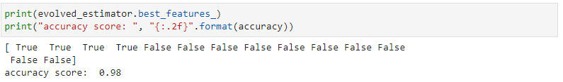
In this run, the test accuracy was approximately 0.98.
The support_ attribute is a boolean mask. Each position corresponds to a
column in the input data: True means the feature was selected, and False
means it was discarded. In this example, the optimizer selected the informative
Iris features and ignored the random noise features.
You can plot the fitness evolution for the feature-selection search too:
plot_fitness_evolution(evolved_estimator)
plt.show()
This concludes the basic sklearn-genetic-opt workflow. The next tutorials cover callbacks, custom callbacks, schedulers, reproducibility, MLflow integration, outlier detection, and cross-validation behavior in more detail.